Research Note: How can we pre-estimate sample size for multi-factorial ANOVA(ANCOVA) designed study?

Question:

Researchers, especially in the field of experimental psychology are still confused with how to estimate the required sample size of a complex design, for example, $2\times 2 \times 2$ between-within mixed design ANOVA, or a more complicated one like, $2(between-subjects)\times 2(between-subjects) \times 2(within-subjects) \times 2(within-subjects)$ . By using which tool/packages could meet this demand does matter.

Thus, the aim of this note is to figure out the most proper(practical) way to estimate the required sample size of mixed design experimental study.

1. Background

We have to review how researcher estimate required sample size for a complex-design study first, and suggest the gap between theorized “power” and its application in research practice.

1.1 On power analysis

First of all, let us review the notion of power analysis. In most case, power of a binary hypothesis test is the probability that the test correctly rejects the null hypothesis when a specific alternative hypothesis is true (see table below).

	$H_0$ is True	$H_0$ is False
Rejects $H_0$	$\alpha$	$1-\beta$
Rejects $H_1$	$1-\alpha$	$\beta$

Here, we could also explain “power” with Signal Detection Theory. For example, regarding $\alpha$ as the probability that one detected a signal even such signal did not appear ( $H_0$ is true), and such situation is also called as “false alert” (Type I error). In the line with this metaphor, we could also assume that $\beta$ could reflect the probability that one did not detected signal, although the signal did presented ( $H_0$ is False), similarly, such situation could be considered as a “miss” (Type II error). Considering the significance level $\alpha$ as a global threshold of acceptance on the probability of Type I error, while $\beta$ as the threshold of accepting Type II error, $1-\beta$ could be captured as the capability of the system does not miss the signal. The notation I mentioned previously is also as known as Neyman-Pearson framework which could be very useful when we are choosing model in practice.

Since we are already familiar with understanding $\alpha$ , and might have been trained during the practice in certain research as that when $p$ value is less than $\alpha$ , the difference could be considered as significant. With the same line of capturing $\alpha$ , another index to reflex the capability of “no miss” is excepted to be larger than $1-\beta$ . Cohen (1988) suggested a set of “pure” numbers, which are free of original measurement unit and could easily computed with collected data.

The simplest and well-known index might be Cohen’s $d$ ,

d = \frac{m_A-m_B}{\sigma}

where, $d$ is the Effect size index for $t$ tests of means, $m_A$ and $m_B$ are population means expressed in raw and $\sigma$ is the standard deviation of either population. The index reflect the aim of Cohen’s attempt on “pure” numeric scaled index with the actual explanation which could corresponded to probability of $1-\beta$ . Thus, we could also take a practical view on general notion of “power” as the ratio of “signal” and “noise” rather than a mathematical one.

It is worth noted that when a researcher is going to conduct power analysis, the definition of “power” should be assumed first. In the case of simple comparison between means of two groups, it could be reflected as the ratio of finite difference on total standard deviation. However, in the case of mixed designed ANOVA, although the general notion of “power” remains still, the power of main effect and interactions, the power on which measures differ on mathematical expressions. I will discuss this in the session 1.3.

1.2 How to compute required sample size

In most time, we could easily compute required sample size for simple situations like one sample, matched sample or two independent samples. For example, in the case of continuous dependent variable one sample test, effect size is defined as $d = \frac{|\mu - \mu_0|}{\sigma}$ , to meet the threshold of significant level and power, required sample size are always given as the following:

n = (\frac{Z_{1-\alpha/2} + Z_{1-\beta}}{effect\ size})^2

where effect size is depended on which test researchers have chosen, for two independent samples and matched samples, effect size are $|\mu_1=\mu_2|/\sigma$ and $\mu_d/\sigma$ respectively. It is also notable that $n$ here refers to sample size per cell, if you are testing two independent samples, the final required sample size should be doubled.

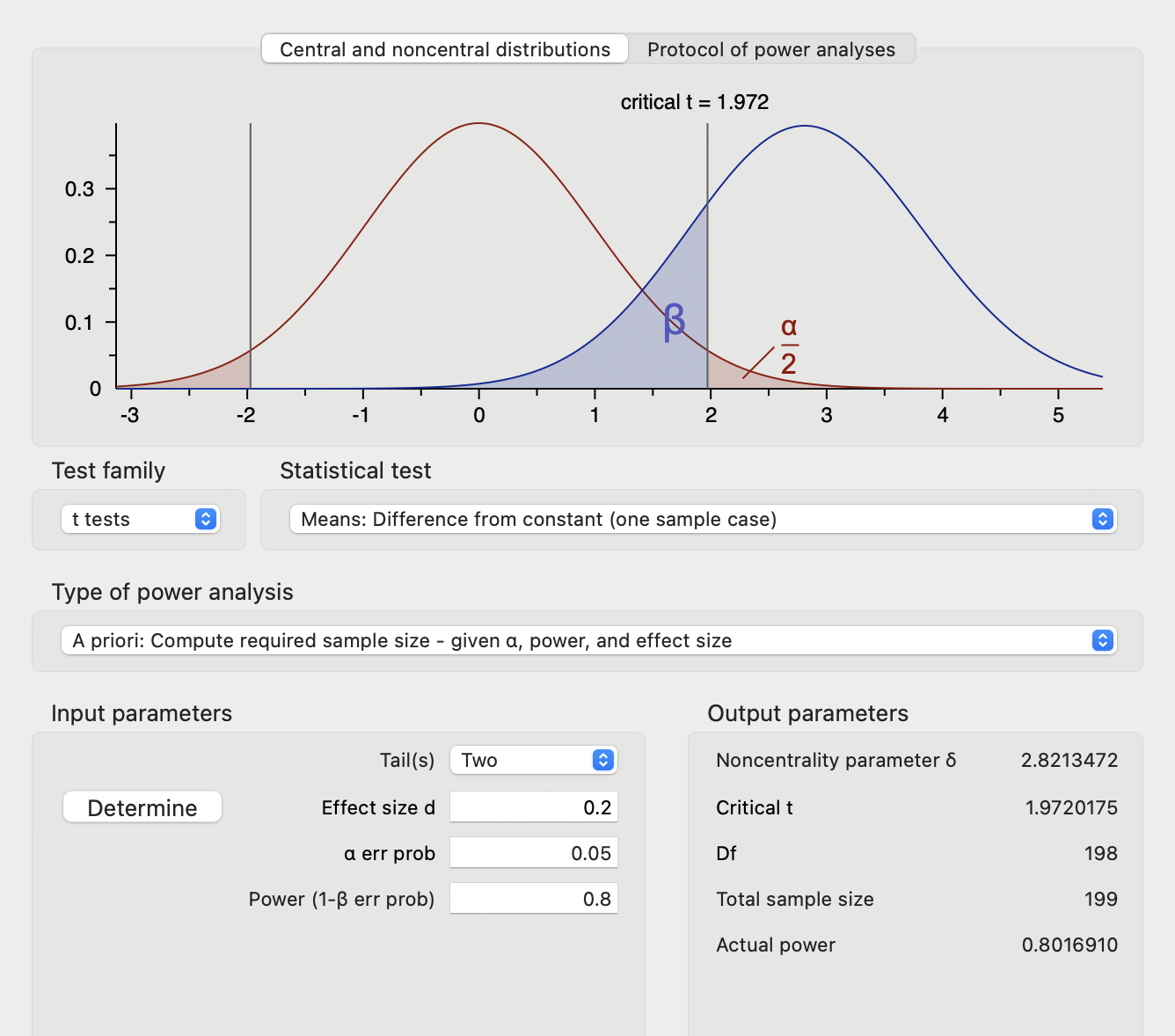
Since all parameters, namely $\alpha$ , $\beta$ and desired $effect\ size$ are determined in previous formula, we could even easily compute it without 3rd party packages in R or Python. Here I provide simple codes with R and we could also compare the result with popular package pwr and G*Power 3.1. Let us set significant level $\alpha$ as 0.05, power $\beta$ as 0.8, effect size as 0.2, and calculate required sample size for one sample case test. Following code block shows that sample size is 197.

calculateSampleSize <- function(effectSize, power, sigLevel) {
  # Convert power to z-score
  powerZ <- qnorm(1 - power, lower.tail = FALSE)

  # Convert significance level to z-score
  sigZ <- qnorm(sigLevel / 2, lower.tail = FALSE)

  # Calculate sample size
  n <- ((sigZ + powerZ)^2) / (effectSize^2)

  # Return the sample size for each group
  return(ceiling(n)) # use ceiling to round up to the nearest whole number
}

# let effect size = 0.2, power = 0.8 and significant level = 0.05 
sampleSize <- calculateSampleSize(0.2, 0.8, 0.05)

print(sampleSize)

# output is 197

Respectively, setting up Test family as “t tests”, Statistical test as “Means: Difference from constant (one sample case)” and Input parameters as same as code above. Total sample size was 199 and it was similar to the output of our simple R script with pwr.

Fig 1

Although the conceptualization of effect size for ANOVA is similar with t-test, things become different due to a vary way when capturing “difference” mathematically. Even the origin inspiration of statistics testing could be described as finding which model fits the reality best, different definition or measurement of objects making it totally different.

1.3 Why estimating required sample on mixed-design study is confusing (annoying)?

Unlike $t$ test or $\chi^{2}$ test, mixed design studies usually involves ANOVA or GLM to test whether hypothesized model is significant first, and then test interested main effects or interaction in the lines with the hypothesis one by one. Thus, not only the calculation of effect size, but also “a priori” which estimate the required sample size always “floating” due to different interests.

First of all, let us review how ANOVA works, and figure out the “signal” and “noise”. As we all know, in one-way ANOVA (assuming we got $i$ levels with total sample size as $j$ ), we could use following formula (structural model) to describe and further provide the mathematical scaffold to test our hypothesis:

x_{ij} = \mu + \tau_{i} + \epsilon_{ij}

where, $\mu$ is the mean overall, $\tau_{i}$ is the effect of condition, $\epsilon_{ij}$ is the error of each sample. We could demonstrate that, $x_{ij}$ (representing the statistical traits of dependent variable) is captured as visible and concrete part $\mu$ , hypothesized effect of any categorical variable $\tau_i$ and error $\epsilon_{ij}$ that could not be observed. Here, I would like to pass some assumptions (e.g., the unbiased inference on $\sigma_{total}^2$ is $E(MS_{total})$ ) on the traits of $\mu + \tau_i$ , just keep in mind that the core notion of ANOVA is using $\sigma_{Total}$ , $\sigma_{m}$ and $\sigma_{error}$ to reflect the uncertainty (or on the other hand, certainty) of $x_i$ , $\tau_i$ and $\epsilon_{ij}$ . Considering we could only using limited sample to estimate $\sigma$ , we have:

SS_{Total} = SS_M + SS_{error}

Since, each part of structural model comes from different view on how to categorize data. Those different blocking data view get different weights to explain the uncertainty of data. Thus, we have to average extent of explaining uncertainty of data within their own dimensions (degree of freedom). Like $t$ is ratio of difference on estimated population standard deviation, $F$ is also a ratio:

F = \frac{SS_M}{df_M}/\frac{SS_{error}}{df_{error}} = \frac{MS_M}{MS_{error}}

Now, what is “signal” and what is “noise”? According to Cohen (1988), the index that reflect the effect size should keep in the line with “free of measurement unit” and “express as averaged effect”, thus, as a generation to $d$ , effect size index for ANOVA is given by figuring out the ratio of uncertainty of measurement to uncertainty of error first, thus here comes index $f$ :

f^2 = \frac{\sigma_m^2}{\sigma ^2}

where, $\sigma_m$ is the mean of the deviation of $i$ levels, as the following relationships between variances,

\sigma_{Total}^2 = \sigma_{m}^2 + \sigma^2

and keeping the conception of effect size as “ratio of the variance of specific measurement/manipulation to total variance”, we could now define $\eta^2$ as following:

\eta^2 = \frac{\sigma_m^2}{\sigma_{Total}^2} = \frac{\sigma_m^2}{\sigma^2 + \sigma_m^2}

with simple algebraic manipulation, we could got:

\eta = \sqrt{f^2/(1+f^2)}

In summary, as same as the difference between $d$ (ratio of difference on total variance) and $t$ (ratio of difference on mean variance). In the case of ANOVA, compared to test statics $F$ (ratio of mean squares of manipulation to mean squares of error), $\eta^2$ could reflex proportion of total variance which is corresponded to the concept of effect size.

1.4 Mixed-design ANOVA with example: repeated measure ANOVA vs. ANCOVA ?

We have followed up with Cohen and summarized the indexing of effect size of one-way ANOVA so far. Finally, the problem showed up, how it comes to mixed-design ANOVA? We have extend more factors of design,

Example

Underlying same principle, we should add more items in a structural model. Let us take an example, assuming a researcher plans to collect data from a $2\times2\times2$ within-between designed study. There are three factors, two of them are between-subject, and one is repeated measurement (as a within-subject factor). A dummy data structure is as below.

Subject	Condition	Gender	Measurement	Score
A	Manipulation	Male	Scale 1	…
A	Manipulation	Male	Scale 2	…
B	Manipulation	Female	Scale 1	…
B	Manipulation	Female	Scale 2	…
C	Control	Male	Scale 1	…
C	Control	Male	Scale 2	…
D	Control	Female	Scale 1	…
D	Control	Female	Scale 2	…
…	…	…	…	…

In such case, we could give two structural models with mixed-design ANOVA and ANCOVA.

Structural model of repeated measures ANOVA

After researching across textbooks and articles, I found that researchers usually do not consider testing within-between interaction as critical. We could use following model to describe the experiment design:

x_{ij} = \mu + c_{i} + \gamma_{j} + (c\gamma)_{ij} + \epsilon_{ijr}

where, $c$ and $\gamma$ represent the main effects of Condition and Gender. For the repeated measurement is defined as $r$ , thus we could figure out that the total sample size is $n = i*j*r$ . Then, we could easily list F-value as following:

Factor	Sum of Sq.	df.	Mean of Sq.	F
$A$	$SS_A$	$df_A=i-1$	$MS_A=SS_A/df_A$	$MS_A/MS_E$
$B$	$SS_B$	$df_B=j-1$	$MS_B=SS_B/df_B$	$MS_B/MS_E$
$A\times B$	$SS_{A\times B}$	$df_{A\times B}=(i-1)(j-1)$	$MS_{A\times B}=SS_{A\times B}/df_{A\times B}$	$MS_{A\times B}/MS_E$
$E$	$SS_E$	$df_E=ij(r-1)$	$MS_E=SS_E/df_E$

Since we ignore the effect of Measurement, original design with $2\times 2\times 2$ between-within factors has changed into pure within-subjects designed one. However, if we do concern about within-between interaction in this example? According to Maxwell & Delaney (2004), a rough but useful approximation of the sample size needed is provided as following:

N_{within} = \frac{N_{between}(1-\rho)}{\alpha}

where $\alpha$ is the number of within-subjects levels and $\rho$ is the correlation between measurements.

Structural model of ANCOVA

We could consider Scale 2 as target variable, and Scale 1 as a covariant:

y_{ijk} = \mu + c_{i} + \gamma_{j} + c_{i}\tau_{ijk} + \gamma_{j}\tau_{ijk} + (c_{i}\gamma_{j})\tau_{ijk} + \epsilon_{ij}

or we could transfer formula as

y_{ijk} = (\mu + c_{i} + \gamma_{j}) + [c_{i} + \gamma_{j} + (c_{i}\gamma_{j})]\tau_{ijk} + \epsilon_{ij}

1.5 Questions emerges: `StackExchange`

When exploring information about the correct usage of G*Power, I found following Question posted 2 years ago. A user of G*Power found inconsistency between the results of Repeated Measures ANOVA and ANCOVA underlying same clinical trials design (original link: https://stats.stackexchange.com/questions/535159/gpower-difference-in-sample-size-for-ancova-vs-repeated-measures-anova-in-clin).

The Inputs are as following:

# ANCOVA
- Effect size f = 0.25
- Sig.level = 0.05
- Power = 0.8
- Numerator df = 1
- Number of groups = 2
- Number of covariates = 1

# repeated measures ANOVA
- Effect size f = 0.25
- Sig.level = 0.05
- Power = 0.8
- Number of groups = 2
- Number of measurements = 2
- Corr among rep measures = 0.5
- Nonsphericity correction = 1

The results were different, although noncentrality parameter $\lambda$ , critical F and actual power were approximate, total sample size calculated by ANCOVA (128) was over 3 times than repeated measures ANOVA (34). Which one is correct?

Misunderstandings and misuses

The situation mentioned above is a common misunderstanding of using popular tool, namely G*Power to calculate the required sample size.

One step forward? Swift ANOVA power analysis question into Generalized Linear Model might help

Although the main stream of testing psychological effect now focusing on simple designed study, it is also necessary to make it clear with how to use power analysis tool to estimate the required sample size and evaluate the effect size with complex mixed-design studies.

Mixed model ANOVA or multi-variable ANCOVA could be regarded as equal to generalized linear model(GLM). Thus, the question I discussed above could also be solved alternatively by conducting the power analysis on GLM. However, this session might deviate from the core concern of this note, I would like to write another note for it.

2. Solutions:

Following solutions are recommended:

use R package pwr and correctly set up the params with error
use G*Power without misunderstanding the parameter settings

Steps by using `pwr`

Steps by using `G*Power`

In G*Power, estimating required sample of a study is called as “A priori” analysis, where sample size N is computed as a function of power level, significance level, and the to-be-detected population effect size.

Let us jump to the parts of F test and multi-regression.

3. Conclusion

In this note, I first viewed the idea of power analysis and how to calculate effect size and required sample size. Then I provided different ways to calculate required sample size for complex mixed-design study by using popular open access software or packages. Finally, for those 3 factorial mixed-design ANOVA, I suggested to transfer model into $2\times 2$ ANCOVA to calculate required sample size and for such multiple factorial ANOVA model over 4 factors, I suggested to regard them as general Gaussian linear model to calculate required sample size.

Keywords: #statistics #power_analysis #ANCOVA